Introduction
WebSPN software tool consists of two main parts:
- user interface: allow the user to specify the Petri net that one wants to study, by simply drawing it on the screen, and to specify the measures of interest
- the analysis engine: analyses the net and computes the measures required by the user.
Measures over a Petri net model are defined through a native language embedded in the tool. A brief introduction can be found in the Measures Help section.
User Interface
The main purpose of the development of the user interface was the ease of use (that is, to give the user the opportunity to operate simply and intuitively). Another purpose was the coherence of the possible operations, and the consistency of the obtained results.
Once the program has been started, it appears as in the figure:
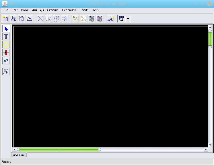
Several zones can be recognized in it:
- bar of menus
- control bar
- component bar
- status bar
- area of design
- tabbed pane
Menu bar
It contains the classical choices of a graphic environment as File, Edit and Help and those more specific as Draw, Analyse, Options, Schematic and Tools. There is a button in the control bar or in the bar of components, for the most frequently used functions.
Control bar
The main operations of menus File, Edit, Analyse and Option can be immediately accessed.
The functions of the buttons are as follows:

Components bar
The items of menu Draw can be immediately accessed. The meaning of each button is:

Status bar
A message of description of the current operation and/or any suggestions about the correct use of the program are viewed.
Area of design
The user can design its own Petri net. It is also possible to see a non visible part of the area by using the scrollbars. The Area of design is delimited by a white border resizable.
Tabbed pane
It allows the user to visualize on the same area of design more Petri nets by switching among opened projects. Click on the corresponding tab to make the corresponding project active.
How to use WebSPN GUI
The first step is to design a Petri net (which represents the model to study). The design of the net is made by selecting the elements of the components bar, and putting them in the area of design (by clicking on it).
Only places, transitions or labels can be inserted, while arcs can be drawn only when at least a place and a transition to be connected have been drawn. It is not possible to connect two places or two transitions with an arc. Besides, it is not possible to draw an arc connecting two already connected objects with the same arc direction; instead, it is possible with an arc in opposite direction.
The properties of a component of the net can be changed by selecting pointer from the component bar, and by double-clicking on the component, the dialogue box summarizing the component properties will appear.
Let us examine the dialogue boxes in detail:
- double click on a place:
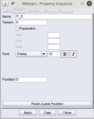
Through this window, the user can specify the name of the place and the initial number of tokens.
N.B. the name must be unique (for analysis reasons), and the number of tokens must be a positive integer. The checkbox Parametric is disabled in the actual release. This function will be available in next software releases.
- double click on transition:
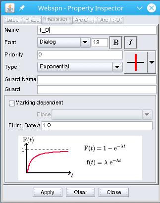
Through this window, a user can set the name of the transition, its priority (if any), its orientation and its type. The specification of the parameters affecting the time behaviour of the transition is linked to the choice of the type. The net will evolve differently, according to the variation of the type of transition.
N.B. The name of the transition must be unique (for analysis reasons), and the priority must be a positive integer or zero. The different specific parameters of each type of transition must be a positive real number (negative times have no sense).
In guard text area you can specify a guard condition associated with the transition.
- double click on an arc:
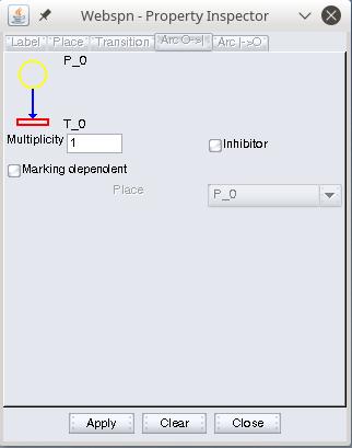 |
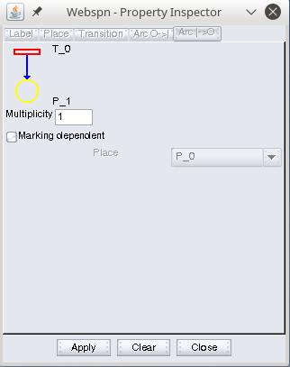 |
The dialog boxes of the arcs are two, depending on whether the arc passes from a place to a transition (figure on the left) or vice versa (figure on the right).
In the upper frame of each dialog, the ends of the arc concerned are indicated. Of course, an arc can be inhibitor only if it passes from a place to a transition.
N.B.The multiplicity field must be an integer > 0, while “marking dependent ” checkbox allows to set arc multiplicity dependent on the number of tokens in a place.
- double click on label
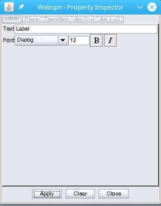
With this dialog we can specify the value of the label, that is, the text that will be read on the screen.
The most appropriate use of a Label is therefore to insert a text commentary in a Petri net. A label can contain any text, even if containing spaces.
Each time the user clicks on a component, he/she selects it and can therefore move it in the area of design and/or cancel, cut, copy it. If one wants to select several components all at once, the select-box can be used, by keeping the mouse button pressed and dragging the mouse till when the components desired are included. By keeping the button CTRL pressed, new components and/or new areas can be selected, without losing the previous selection.The fundamental operations as copy, cut, paste and cancel can quickly be performed through an appropriate combination of keys: Del (cancel), CTRL+C (copy), CTRL+X (cut) and CTRL+V (paste).If one wants to change the state of an arc, the button MoveEdge of the components bar must be pressed. Then we only need to move the handles (of the selected arc), till the form desired is obtained.Arcs can be viewed as piece wise or as spline curves; we can switch from these two types of view, selecting or not selecting Toggle of the element Spline in the Draw menu. If we want to view all the arcs as spline curves only temporarily, we can selecting Show all of the element Spline in the Draw menu. Once the phase of design has been completed, we can proceed to the analysis of the net, by pressing the button Analyse.
Project analysis
The analysis engine is implemented by following the client/server model. The client is included in the design interface, while the server is a demon that waits for requests form outside indefinitely. The client makes sure that the net has an initial marking, and gives the user the opportunity to specify the parameters and desired measures through the following dialog window:
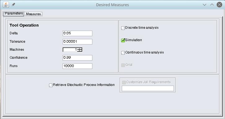
This first tab window allows us to specify:
- Analytical mode for mathematical solution in discrete time, Simulation mode for simulated solution, Symbolic mode for mathematical solution in continous time.
- the step analysis (Delta), that must be lower than the shortest time associated with the timed transitions in the net. This parameter is mandatory for all type of solutions.
- the tolerance (Tolerance), that is the steady state elaboration precision.
- the number of computers (Machine) which will resolve the Petri net. This parameter should be used only if you want to resolve the net by simulated or analytical parallel (MPI) solution.
- the confidence (Confidence), that represents confidence value (you can set it only if you use Simulation mode for analysis).
- the runs (Runs), that represents the numbers of times that you want to simulate the net (only for Simulation mode).
- the retrieval of some intermediate analysis files, such as the ReachabilityGraph and the StateProbability file. The first file contains the reachability graph of the model; the second one stores the probabilities of the all states.
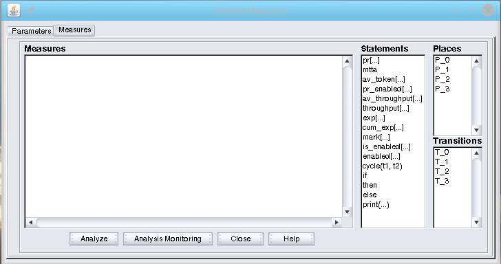
The second tab window allows us to specify:
- the measures required (Measures), which must be written by following an appropriate syntax specified in the Help. A double click on an item in Statements, Places, Transitions causes it to be inserted in the area of editing of the measures, in the current position of the cursor.
By pressing the Analyze button the client communicates with the server, sending the data necessary for the analysis.
By pressing Analysis Monitoring button the user can monitor the completed and running analysis and simulation by following window:
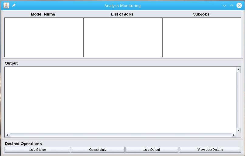
The window consist of:
- Model Name area that shows the Petri net model launched on the server.
- List of Jobs area that shows a list of different execution of the same model.
- Output area that is used to show the information resulting by interaction with button set.
- Job Status button is used to display the current state of selected job.
- Cancel Job button is used to delete selected job from the server.
- Job Output button is used to retrieves .tgz result file.
- View Job Details button is used to display the startup parameters and measures of selected job.
Measures Help
- Available measures:
- How to define a Reward Function f:
- How to define <event>:
- Example of valid statement:
- Possible mesasures:
- pr[Event]
- steady state probability of Event
(return a value) - pr(time)[Event]
- instantaneous probability of Event
(return a value) - cycle(time1, time2 [, step]) pr[Event]
- probability of Event in interval [time1, time2]
(return an array of values)
- av_token[Place Name]
- steady state average number of tokens in Place Name
(return a value) - av_token(time)[Place Name]
- instantaneous average number of tokens in Place Name
(return a value) - cycle(time1, time2 [, step]) av_token[PlaceName]
- average number of tokens in Place Name in interval [time1, time2]
(return an array of values)
- pr_enabled[Transition Name]
- steady state probability that Transition Name is enabled
(return a value) - pr_enabled(time)[Transition Name]
- instantaneous probability that Transition Name is enabled
(return a value) - cycle(time1, time2 [, step]) pr_enabled[TransitionName]
- probability that Transition Name is enabled in interval [time1, time2]
(return an array of values)
- exp[Reward Function]
- steady state expected reward rate of Reward Function
(return a value) - exp(time)[Reward Function]
- instantaneous expected reward rate of Reward Function
(return a value) - cycle(time1, time2 [, step]) exp[Reward Function]
- expected reward rate of Reward Function in interval [time1, time2]
(return an array of values)
- cum_exp[Reward Function]
- steady state expected accumulated reward rate of Reward Function
(return a value; available only if the Petri Net have absorption markings) - cum_exp(time)[Reward Function]
- instantaneous expected accumulated reward rate of Reward Function
(return a value) - cycle(time1, time2 [, step]) cum_exp[RewardFunction]
- expected accumulated reward rate of Reward Function in interval [time1,time2]
(return an array of values)
- mtta
- Mean Time To Absorption
(return a real value; available only if the Petri Net has absorbing markings)
f := <Reward Function Expression> or <Conditional Reward Function Expression>
(f is an array of values)
- <Reward Function Expression>:
- a numerical expression in which the only functions allowed are:
- mark[Place Name]
- return the number of tokens in Place Name
(return an array of values) - enabled[Transition Name]
- return 1 if Transition Name is enabled, 0 otherwise
(return an array of values)
- <Conditional Reward Function Expression>:
- an IF THEN ELSE statement in the following form:
if <Event> then <Reward Function Expression> else <Reward Function Expression>
(ELSE clausole is not optional)
The numerical expression consist of an algebric expression with parenthesis and the following operators (the order represents the precedence too):
– : unary minus
^ : power operator; is considered left associative
2^3^4 is evaluated as (2^3)^4, not 2^(3^4). To specified a specific evaluation order use the parenthesis.
*, /
+, –
Is a boolean expression with parenthesis and the following operators (the order represents the precedence too):
- ! : not
- & : and
- | : or
The basic event have one of the following form:
- #PlaceName <RelationalOperator> <numerical expression>
- mark[PlaceName] <RelationalOperator> <numerical expression>
- ?TransitionName
- is_enabled[TransitionName]
- Note:
- # and mark are equivalent
- ? and is_enabled are equivalent
- The relational operators are:
- ==
- <
- <=
- >
- >=
- !=
Each expression that a user can define must be assigned to a variableto view the result of expression or to use the result in other expression.
There are two types of assignment, a value assignment and an array assignment.
If the expression value is a value, the form of assignment statement is:
variable_name = expression
If the expression value is an array of values, the form of assignment statement is:
variable_array_name := expression
To view the value of one or more variables that represent a value (NOT AN ARRAY) the PRINT keyword must be used, i.e.:
print(a, b, ...)
The arrays obtained by means of CYCLE keyword are automatic visualized in the result dialog.
If an array represents a REWARD FUNCTION only the relative expected reward rate and expected accumulated reward rate can be viewed.
How to calculate and view the steady state average number of tokensin a place:
m1 = av_token[PlaceName]
print(m1)
How to calculate and view the instantaneous average number of tokens in a place:
m1 = av_token(7)[PlaceName]
or
t = 7
m1 = av_token(t)[PlaceName]print(m1)
How to calculate and view the Mean Time To Absorption (MTTA):
(mtta is calculated only for Petri Net with absorption marking)
t = mtta
print(t)
How to calculate and view the steady state probability of an event:
p = pr[#place1>0 & #place2=0 | #place3==5]
print(p)
How to calculate and view the instantaneous probability of an event:
p = pr(15)[#place1>0 & #place2=0 | #place3==5]
or
time = 15
p = pr(time)[#place1>0 & #place2=0 | #place3==5]>print(p)
How to calculate and view the steady state probability that a transition is enabled:
p = pr_enabled[TransitionName]
or
p = pr[?TransitionName]print(p)
How to calculate and view the instantaneous probability that a transition is enabled:
p = pr_enabled(20)[TransitionName]
or
time = 20
p = pr_enabled(time)[TransitionName]print(p)
How to define a reward function:
f := mark[PlaceName]
or
f := enabled[TransitionName]
or
f := if mark[PlaceName]>0 then 1 else 0
or
f := if mark[PlaceName]>0 then mark[PlaceName]*10 else mark[PlaceName]/10
How to calculate and view steady state expected reward rate of a reward function:
p = exp[f]
print(p)
How to calculate and view steady state expected accumulated reward rate of a reward function:
p = cum_exp[f]
print(p)
How to calculate and view instantaneous expected reward rate of a reward function:
p = exp(25)[f]
print(p)
How to calculate and view steady instantaneous accumulated reward rate of a reward function:
p = cum_exp(10)[f]
print(p)
How to calculate and view the value of a measure in interval [t1, t2]
v:=cycle(t1, t2 [, step]) pr[#PlaceName >=0]
or
v:=cycle(t1, t2 [, step]) av_token[PlaceName]
or
v:=cycle(t1, t2 [, step]) pr_enabled[TransitionName]
or
v:=cycle(t1, t2 [, step]) exp[RewardFunction]
or
v:=cycle(t1, t2 [, step]) cum_exp[RewardFunction]
step is optional; if it is not present or is lower then delta it is set to delta
IMPORTANT: each statement must be written in a single line!!!
i.e.:
a = pr[ #p_0>0 & is_enabled[t_1] ]
is correct, while:
a = pr[ #p_0>0 &
is_enabled[t_1] ]
is wrong.
Implemented measures
|
MEASURES |
ANALYTICAL |
SIMULATION |
SYMBOLIC |
|
pr |
• |
• |
• |
|
pr_enabled |
• |
• |
• |
|
av_token |
• |
• |
• |
|
exp |
• |
• |
• |
|
cum_exp |
• |
• |
• |
|
mtta |
• |
• |
• |
|
throughput |
• |
||
|
av_throughput |
• |

